|
|
|
|||||||||
|
||||||||||
|
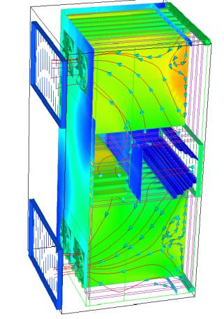
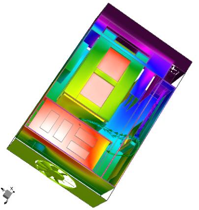
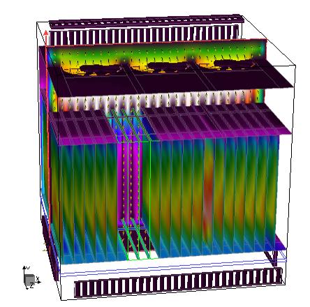
The 3.5-kW
device was designed by CAS Ltd. and built by Charlottes Web Networks Ltd.
Having gained experience with thermal software by following the modeling tips
in this article, engineers with the companies optimized the product for
smallest size. CFD optimization in software called Coolit from Daat Research,
let the company trim the number of anticipated fans by creating the optimal
airflow in the system with judicious placement of components, boards, and
vents. All this was done without building physical prototypes. Specialized computational fluid dynamics or CFD software provides a wide range of capabilities for computer prototyping of electronics in enclosures. The software lets thermal engineers shorten design cycles, and eliminate building and testing physical prototypes. The software also lets designers quickly and efficiently evaluate "what if" scenarios, it simulates conditions not reproducible in a lab, and provides more detailed information than do lab experiments. Finally, the technology improves the operation and endurance of electronics and optimizes placement, size, and parameters of components. In short, it helps get a design right the first time. CFD
technology involves solving transport equations of fluid flow and heat transfer
on computers. To solve the equations, they must be represented so computers can
handle them. This is usually done with so-called finite volume or
finite-element methods. The latter were successful only in specialized CFD
applications, such as slow flows and non-Newtonian flows. Most all production
CFD programs currently use finite-volume methods and we will refer only to
them. Putting
the latest CFD technology to best use takes practice and a few unavoidable
mistakes. The problems here are solved with software called Coolit from Daat
Research and the following guidelines have been compiled from observations of
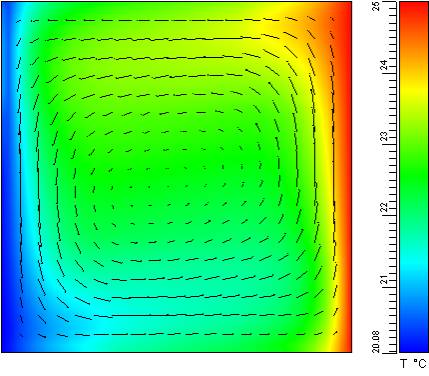
new users. Learning from their mistakes may shorten your learning curve. Start with simple models. Gain confidence in your modeling abilities and the softwares capability, start with simple problems, and compare results to analytical solutions and experimental data. One of the easiest problems to set up includes laminar natural convection in a square cavity with vertical heated walls and adiabatic conditions at top and bottom. The
problem should take a few minutes to set up and even less to solve. A solution to this problem appears in the
accompanying illustration Flow in a
square cavity. The same problem can be slightly modified to obtain another
well-researched solution of turbulent natural convection in a rectangular
cavity.
To get familiar with the
software and build confidence in its use, work on simple well-documented models
such as the flow in a square cavity with heated walls. Finding
out how your numerical solution stacks up against the real world is easy with these
examples because readily available reliable data makes for an easy comparison.
If you experimented with the model by setting different grids and convergence
criteria, you noticed the solution changed along with the parameters. Determining a sufficient grid
for an accurate numerical solution means finding the coarsest grid or mesh that
provides good answers. This discussion applies both to unstructured and
structured grid systems. In general, a finer grid produces more accurate
solutions than a coarser one on the same models. In mathematical terms, the
numerical solution will tend to the solution of the underlying partial
differential equations as the grid is refined. In
practice, however, a uniform grid refinement for 3D problems is virtually impossible
as the total number of grids grows exponentially. For instance, if a model has n = 70 grid cells in each direction,
increasing the number by only 10% will increase the total number of grid cells
33% from 343,000 to 456,533. Increasing n
by 50% in each direction expands the grid to over a million cells for a 238%
growth.
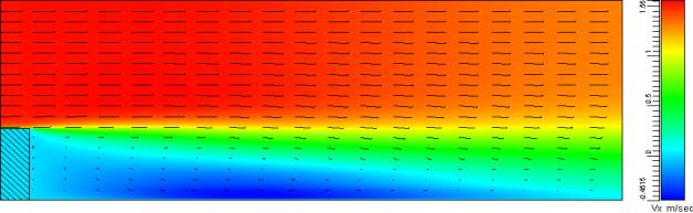
Another simple
but important problem is the backward-facing step flow. In fact, every obstacle
in the path of airflow is a backward-facing step. Many experimental and
numerical results are available for comparison. Fortunately,
the solution error depends on both the total number of grid cells and their
distribution. Correctly distributed grids go a long way toward getting an
accurate solution. A simple example illustrates the point. Consider an
exponentially fast varying boundary layer, which is obtained as a result of
solving a convection diffusion equation:
Solving
this problem on uniform grid with R=10
produces 14% maximum error when 10 cells are used in the boundary layer. To
reduce that error to less than 5%, at least 100 uniform grid cells are needed
in the boundary layer.
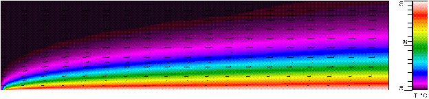
The image is an example of a
laminar temperature boundary layer developing on a flat plate. Its another
important problem because its encountered frequently, its easy to set up, and
solutions are readily available. A
better way to reduce the error is to use non-uniform grids, with smaller cells
towards the wall, where the solution changes rapidly. In the case of the
boundary layer, an optimum solution uses a logarithmic distribution of grids.
Such grid will yield the exact solution with only two cells in the boundary layer!
Obtaining
exact solutions on specially designed grids is not an easy feat for general 3D
problems. Sufficiently accurate grids, however, are possible. Software, such as
Coolit, will automatically produce grids optimized in that regard. But
the question still remains: In the absence of experimental data, how can one
determine a sufficient grid? The only method is to recompute the same problem
on finer grid and compare results. When the solution in the points of interest
does not appreciably change, the previous grid was sufficient. Otherwise,
youll need to repeat the process until changes to the solution become small. Define the simulations goal before you
start modeling.
A goal could be to reduce the number of fans, keep the temperature of a
particular package or component within limits, or select a heat sink.
Objectives change as projects progress. Use
coarse grid simulations to determine the sensitivity of design decisions on
critical components, such as fan parameters or placement. The same applies to
optimization problems that require comparing different designs to find a best
one. This case would call for examining relative rather than absolute numbers.
If an objective is to determine heat-transfer coefficients on the surface of an
enclosure, there is no need to specify internal details. The only important
element is the position and power of heat sources. The accuracy of a predicted
heat transfer coefficient would not be affected. Do a triage on your CAD model.
In most cases, one cannot simply press a button and move a CAD model to thermal
software. Too much detail overwhelms computers without a corresponding
improvement in accuracy. Simplify the model by deciding what is important in
the simulation. For example, consider an enclosure with several pin fin heat sinks, each with 11x11 pins. A coarse grid - about two grid cells per pin, three per space between the pins, and 20 cells in the direction normal to the base - requires 500,000 grid cells. Add other components and you quickly run out of computer resources. Ask
if the model needs an accurate solution everywhere, or only in certain parts of
the model. Be realistic. Greater accuracy requires more time to build a more
detailed model and finer grid with correspondingly longer solution times. Its
worth the effort to trade unneeded detail in a model for a shorter solution
time. With regard to pin-fin heat sinks, when its critical to find a solution
around only one sink, then replace the other two with lumped-parameter
versions, such as a porous media model available in most CFD codes. The effect
of the lumped-parameter heat sinks on the rest of the problem should be close
to that of the detailed model, so the solution around the important sink is not
adversely affected. Dont forget that partially converged solutions are one way
to quickly check a model setup for its accuracy. A complex model usually takes
considerable time to reach a fully converged solution, and a mistake in the
setup wastes that time. Instead, solve the problem for a few iterations
and look at results. Recognizing modeling errors early allows correcting them
before the case converges. You may, for example, see that a component is
unexpectedly hot - a good indicator that you mistyped its power dissipation or
thermal conductivity value. Or, check the fan curves when a flow seems too
fast. Its a good idea to use this technique every time you start a complex
model.
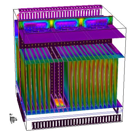
The avionics equipment built
by Miltope Corp. Boulder, CO, was also optimized using CFD software. The model
used several lumped parameter submodels and successfully predicted temperatures
of critical components to within a few degrees.
The heat sinks look similar but analysis with CFD software showed that one is 50% less efficient than the other. Reports accompanying the analysis further detail the study with quantitative information. Use a coarse-grid solution when faced
with optimization or sensitivity studies. Looking for an
optimum component arrangement usually requires comparing several different designs
to determine their relative performance. Coarse-grid analysis is the perfect
tool for the task. It allows quickly and efficiently predicting whether one
design is better than another. NEC engineers, for example, used the method to
quickly determine that a heat sink from one manufacturer is 50% less effective
than a similar one from another. Sensitivity
studies with coarse grids make sense when you dont have all the information to
build a CFD model, or when some of the information is suspect. It becomes
important to determine whether or not the suspect quantity appreciably affects
the prediction of critical parameters. When it turns out the missing data is
unimportant, the analyses can safely continue using estimates. The
same approach works when its necessary to determine sensitivity to lumped
parameter models. After replacing a component or a group with their simplified
versions, it is important to determine how the change affects critical parts.
Coarse-grid analyses let users judge whether important components in the model
are sensitive to the parameters selected for the lumped parameter model. Check the mass and energy balance
using hand-calculated estimates. Its a good way to see whether or not a CFD
model has gross errors. Do the mass and energy balances hold? Does the order of
magnitude predicted using hand-calculations and numerical simulations agree? If
any of these are not true, look for an error in the setup or the model. Identify turbulence.
All CFD programs require that users specify whether the flow is turbulent or
laminar before doing the simulation and, if the flow is defined as turbulent,
require you select a turbulence model. (Turbulence models are approximations of
the original equations that allow simulations on regular grids.) Turbulence
models are necessary because even though the CFD governing equations correctly
capture turbulence, very fine grids are required to do so accurately. This
approach of modeling turbulence on fine grids is called a direct simulation and
is used primarily in academia for basic research. Selecting
the right type of flow is important because assuming laminar flow instead of
turbulent may significantly under-predict heat transfer. Robust turbulent eddy
mixing results in the effective thermal conductivity in electronics
applications ten to hundred times greater than it is for laminar flow. Many
commercial CFD codes provide on-line advice based on specified boundary
conditions. But the advice is often misleading. For example, one suggestion
says when a system has a fan, flow is turbulent. That is indeed true next to
the fan. The question is whether the flow is still turbulent as it goes through
the rack of closely spaced PCBs carrying heat-sensitive components. It probably
is not. Most of the airflow will bypass the rack along paths with less
resistance. And whatever goes through the rack becomes laminar as the flow
squeezes in the narrow passageways between boards. Using
a turbulence model with wall functions is likely to over-predict the amount of
heat transfer from the board. That means the model will predict lower than
actual temperatures for board components. A better choice is to avoid the
turbulence model or use advanced turbulence models without wall functions,
which work reasonably well in both the laminar and turbulent regions of the
flow.
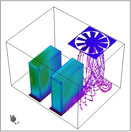
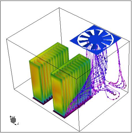
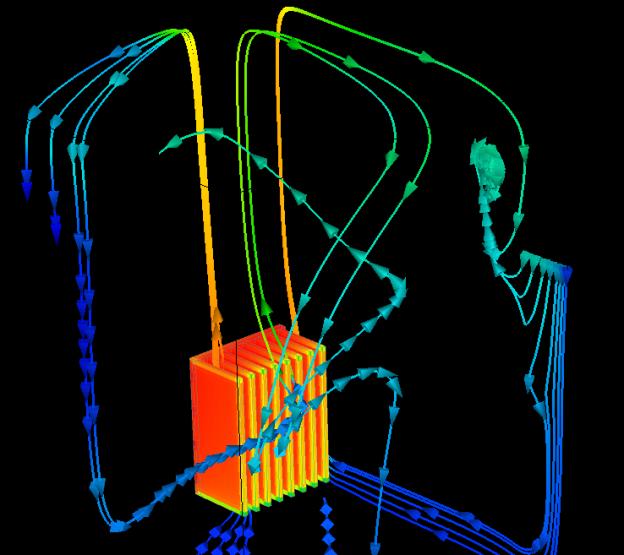
The simulation for an electronics equipment
manufacturer was computed using a turbulence model in Coolit that is capable of
modeling mixed flows. It correctly predicts transition of flow from highly
turbulent (white) to laminar (violet) and again to turbulent. A
special case is free convection flows that have no steady state solution. For
example, in the flow shown below, the air plume at the point of impact where
the rising warm air hits the ceiling of the enclosure oscillates. You wont be
able to find a steady state solution to this laminar flow problem. The solution
residuals, that measure the departure of solution from steady state after
reaching a plateau oscillate with the flow. Users have several options after
recognizing that the plumes oscillations have almost no effect on the
temperature of the plate fin below:. accept the solution with oscillating
residuals as converged; use a turbulence model without wall functions to
dampen the oscillations and obtain a steady state solution, or solve the
problem as time-dependent, obtain results over a period, and average them. All
three approaches are legitimate and produce similar results. But unless you are
writing a scientific paper, the third approach is not practical because it
takes a lot longer than the other methods.
Coolit simulation of the Nokia benchmark
experiment in which a rising plume oscillates. |
||||||||||
|
||||||||||