|
For this paper the flow around a single wall-mounted obstacle was selected. Both
the problem geometry, resembling a building block in electronics and low Reynolds
number flow are characteristic of electronics cooling applications. Due to its
classic configuration, the problem has attracted attention of experimentalists and
reliable data are available to benchmark CFD against.
Experiment
The modeled experiment consisted of a 50 mm high and 600 mm wide wind-tunnel with a
15 mm cube placed on the channel floor along the centerline. To ensure turbulence, the
flow was tripped 75 cm upstream of the cube. The cube was made of 12 mm copper core
coated with a uniform 1.5 mm epoxy layer. The cube’s core was kept at constant
75C. The inlet air temperature was kept at 21C and the average velocity was 4.47 m/s
yielding Re = 4440 based on the cube’s height. For additional details of the
experimental setup and measurement techniques refer to [1, 2].
CFD calculations
The experiment was modeled using Coolit’s four turbulence
models: algebraic [3, 4], differential [5], Secundov eddy viscosity
model [6], and Spalart-Allmaras eddy viscosity model [7]. Results for
k-e model were borrowed from [8] as implemented in the PHYSICA CFD
code [9]. The differential and both eddy viscosity models used
default settings. The algebraic model requires the user to specify
background turbulence level, which serves as the foundation of the
rest of computations. The differential and eddy viscosity models also
require turbulence level, but only as an initial guess, which is then
recomputed by the model.
We estimated the background turbulence viscosity required by the
algebraic model from nt=
sqrt(3/2)uavgIl
,
where the average velocity, uavg = 4.47 m/s,
the turbulence intensity, I, is estimated from the
experimental setup to be approximately 0.05%, and the length scale,
l, is computed from the duct’s height, l = 0.07
H, where H=0.05 m. Thus, nt
= 9.6E-6 m2/s and the background turbulence level,
nt/n=0.64.
Flow Field
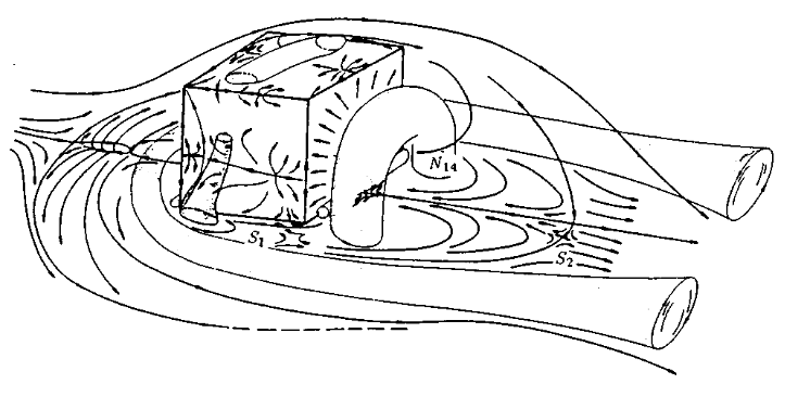
The flow structure around the cube is extremely complicated with
oscillating time-dependent vortical structures on all wetted sides of
the cube. The schematic in Fig. 1 depicts main structures of the flow
[10].
The vortex system starts at the leading edge of the cube with a horseshoe
vortex extending along both sides of the obstacle, a large arch
vortex at the trailing edge, and a separated flow with associated
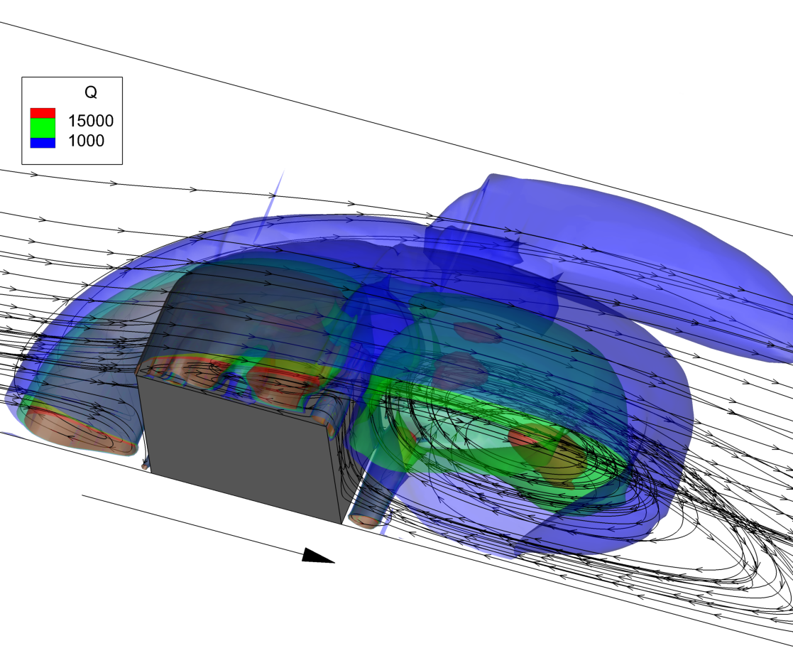
vortices along the top face of the cube. Figure 2 shows
the flow structure computed by Coolit showing Q-criterion isosurfaces outlining the
vortex structure with the section along the channel centerline (Q-criterion
isosurfaces represent local balance between shear strain rate and vorticity
magnitude).
Results
When turbulence models are used, the fine time-dependent flow
structure is averaged to get a smooth steady state solution. This is
what is required for engineering simulations the goal of which is to
predict average flow and thermal characteristics. All the turbulence
models we used were successful in that regard. The question is how
accurate their predictions were for average quantities, which is what
are normally computed in common electronics cooling application
models.
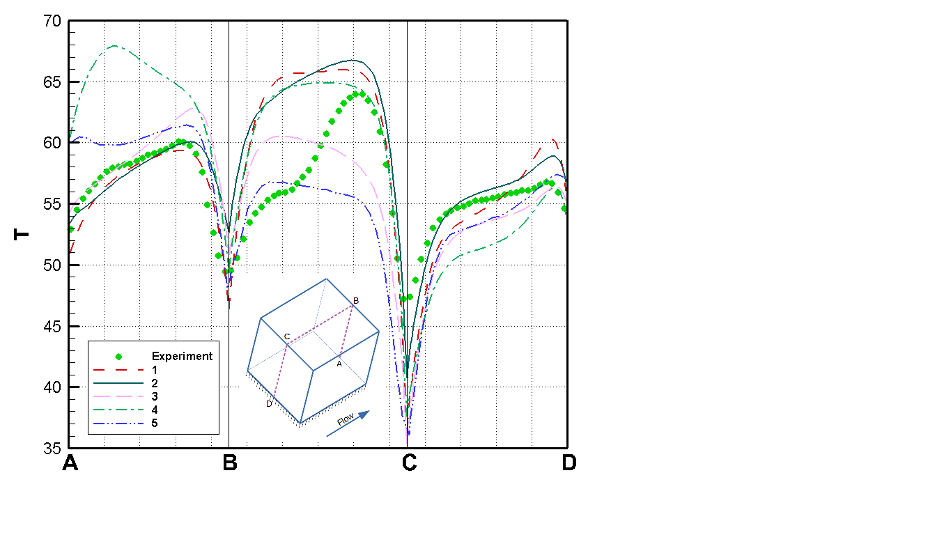
In order to pick some of the flow structures depicted above we
used the 183x101x124 non-uniform mesh. The results computed using 5
different turbulence models predicting the surface temperature along
the ABCD line are shown in Fig. 3 where turbulence models are designated as follows:
1 – Differential [5]
2 – Spalart-Allmaras eddy viscosity [7]
3 – Secundov eddy viscosity [6]
4 – Algebraic [3, 4]
5 – k-e [8, 9]
We also computed the average temperature along the ABCD line:
|
Experiment
|
Spalart-Allmaras
|
Secundov
|
Algebraic
|
Differential
|
Standard k-e
|
|
56.33
|
58.38
|
55.86
|
58.72
|
57.5
|
53.4
|
All turbulence models predicted fairly well general trends of the
temperature. With the exception of Spalart-Allmaras model, the models
somewhat miss the trend on the top surface and the algebraic model
was too hot in the trailing edge area. The average temperatures shown
in the table were also good for all models. All Coolit models
predicted the average temperature rise well under 5% of experiment,
while the k-e model was slightly above 5%. This was the main takeaway
from this study, as detailed computations of turbulence are beyond
the reach of any practical scenario and requirements.
Conclusions
In this paper we compared results from the experimental study [1,
2] with CFD simulations. The problem geometry and the turbulence
level were to resemble typical flow conditions in electronics cooling
applications. Extremely complex flow structure as well as the
temperature prediction in a thin 1.5 mm layer of a low thermal
conductivity material with steep temperature gradients presented a
formidable challenge. We used four turbulence models available in
Coolit and have included for reference results from the popular k-e
turbulence model [9]. Both detailed and average results were good for
both the eddy viscosity and the algebraic models. All Coolit models
predicted the average temperature rise well under 5% of experiment,
while the k-e model was slightly above 5%.
While the algebraic model produced good results, its accuracy
rests on the user-specified background turbulence, which is a
formidable task to predict in real-life applications. In contrast,
eddy viscosity models don’t require such inputs and compute
background turbulence as part of the simulation. The drawback of the
eddy viscosity models compared to the algebraic model is the
computational time and RAM required for solving a partial
differential equation. On modern computers, however, this burden is
minimal and amounts to less than 5% both for computational time and
RAM requirements. Therefore Coolit’s eddy viscosity models are
the optimal choice under most circumstances.
References
Meinders E.R., Hanjalic K., and Martinuzzi R.J., Transactions of
ASME, v. 121, 1999.
Meinders
E.R., PhD Thesis, Delft University of Technology, 1998.
Smagorinsky
J. et al., Monthly Weather Rev., 93(12), 727-733, 1965.
Deardorff
J.W., J. Comput. Phys., 7, 120-133, 1971.
Travis
J.R., Nat. Heat Transfer Conf., Denver, Colorado, Aug. 5-9, 1985.
Gulyaev
A.N., Kozlov V.Ye., and Secundov A.N., ECOLEN ,Scientific Research
Center, Preprint #3, 1993.
Dacles-Mariani,
J., Kwak, D., and Zilliac, G. G., Int. J. for Numerical Methods in
Fluids,
Vol. 30, 1999, pp. 65-82.
Spaulding
D.B., HTS/79/2, Imperial College, 1979.
Dhinsa
K.K., Bailey C.J., and Pericleous K.A., ITherm,
July,
2004.
Hussein
H.
J. and Martinuzzi R. J., Physics of Fluids, vol. 8, pp. 764-780,
1996.
|